7-Mar-2015: Non-constant acceleration

PURPOSE

The purpose of this experiment was to solve a problem analytically and numerically and comparing the results to observe the effectiveness of the numerical model.

PROCEDURES

Analytical Integration

Figure 1: Problem statement

Figure 2: Acceleration function

We began this experiment by deriving an equation for the acceleration based on the conditions given in the problem statement of Figure 1. This acceleration equation is displayed in Figure 2 above.

Figure 3: Velocity function integrated from acceleration function

Next, we found the velocity equation (Figure 3) by integrating the acceleration equation and plugging in initial velocity given in the problem statement.

Figure 4: Integration by parts

Figure 5: Position function integrated from velocity function

We proceeded to find the position equation by integrating the velocity equation that we found in the previous step. However, this integration was much more complicated than the first and required the use of integration of parts (Figure 4). For in depth step-by-step solution of this integration, refer to the lab handout. The resulting position equation is shown in Figure 5.

After finding the necessary equations we found the time at which the elephant came to rest. We did this by setting the velocity equation equal to zero and solving for time. We found this time to be 19.69 seconds. Then, we used this time value to find the elephant's position when it came to rest. We plugged in 19.69 s for t in the position equation and found its position to be 248.7 m.

Numerical Integration

For the next part of the lab, we opened up an Excel file and set up six columns. These seven columns were time (t), acceleration (a), average acceleration (a_avg), change in velocity (Δv), velocity (v), displacement (Δx), and position (x). The time column was arbitrary, but we decided to go to about 20 seconds in intervals of 0.1 seconds (this time interval was established in B1). In order to find the acceleration we input the formula "=-400/(325-A3)" into B3. We then used the Fill Down function to find the acceleration all the way down the column (we used the Fill Down function for all succeeding columns). After filling down the acceleration column, we found the average acceleration values by typing in the formula "=(B3+B4)/2" into C4. Next, we found the change in velocity with the formula "=C4*$B$1," which we placed in E3. The dollar signs were used to establish B1 as an absolute value that does not change. For the velocity at the end of the time interval, we used the equation "=E3+D4" in E3. Then, we found average velocity down column F with "(E3+E4)/2." The displacement was found by inputting "=F4*$B$1" into G3. Finally, we found the position at any given time by plugging in "=H3+G4" into H3. The resulting spreadsheet is shown in Figure 6.

Figure 6: Numerical calculation of the problem

From the figure above, it can be seen that the elephant's position at 19.7 seconds is 248.7 meters, which is very close to the quantity that we found in the previous section. This is due to the fact that we used a time interval of 0.1 seconds, which gave us accurate results. We could have used an even smaller time interval to produce even more accurate results.

CONCLUSION

This lab gave us another tool for solving equations by filling out a spreadsheet in Excel. This can be a very useful tool especially when we come across equations that are very difficult to solve analytically, such as the one we solved in this lab. Sometimes, there are problems that are virtually impossible to solve by hand, which makes this problem-solving method a very powerful tool.

It can be seen how good of a problem-solving method this is by comparing the results that we got from doing the problem analytically and doing it numerically. When we solved the problem analytically, we found that the elephant took 19,69 seconds to come to a stop at a position of 248.7 meters. These values are nearly identical to the ones that we got from solving it numerically: 19.7 seconds and 248.7 meters.

One of the reasons why we got these results is because we chose a time interval that was small enough. We know that the time interval we chose for the integration is small enough by looking at how accurate the results are when comparing them to the results that we found analytically. If we did not have the analytical results to compare to, then we could observe how the values are changing in between time intervals. If we see that there is a big jump from one value to the next, then we know we have to decrease the time interval to find out what is exactly going during that time interval.

16-Mar-2015/18-Mar-2015: Finding the coefficient of friction

PURPOSE

The purpose of this experiment was to use various experimental and mathematical methods to find the coefficient of friction between two surfaces.

PROCEDURES

Part 1: Static Friction

Figure 1: Initial set-up of our experiment

We began the first part of this experiment with the set-up shown in Figure 1 (except we started with one block, not two). We added water to the cup until the block began to accelerate. We then measured the mass of the water and the cup that caused the equilibrium to be broken. We also measured the mass of the block. We repeated this step three times, adding another block each time. The collected data is shown in Figure 2.

Figure 2: Data set

Also displayed in Figure 2 is the normal force acting on the block. We found this by setting up Newton's second law of motion in the y-direction. Since the block was not accelerating vertically, we set the normal force of the block equal to its weight. In other words, we found column three of Figure 2 by multiplying the corresponding values of column one with the acceleration due to gravity: 9.81 m/s² (we used 9.81 m/s² instead of 9.8 m/s² in order to be more accurate with our calculations). After we found the normal force, we determined the maximum static friction force. We accomplished this task by first assuming that the tension in the string that was pulling on the block was equal to the weight of the water and cup system. Then, we assumed that this tension was also equal to the maximum static friction force because it is the amount of force that was required to bring the block out of equilibrium. From these calculated values, we constructed a graph with the friction force on the y-axis and the normal force on the x-axis. The slope of this graph was intended to give us the coefficient of static friction (µ_s), which was 0.2068 in this case. The graph is illustrated in Figure 3 (click to enlarge).

Figure 3: Static friction vs normal force graph

Part 2: Kinetic Friction

After solving for the coefficient of static friction between the block and the track, we attempted to solve for the coefficient of kinetic friction (µ_k) of the same system. To accomplish this task, we used a set-up that was very similar to the one shown in Figure 1. The only modification we made was that we replaced the pulley and cup with a force sensor. We pulled on this force at a constant rate to implement a constant force on the block. Then, we repeated the process three more times, adding another block on top of the first after each trial. The forces that we applied on the blocks are shown below in Figure 4 (click to enlarge).

Figure 4: Graphs of the forces applied on the blocks during each trial

We took the averages of the graphs in Figure 4 to find the kinetic friction force. We once again plotted these forces against the normal forces for each block to find the coefficient of friction from the slope of the graph. We found this value to be 0.2168, which was actually bigger than the coefficient of static friction found earlier. The reason why this may have been so will be discussed later in the conclusion. This graph is displayed in Figure 5 (click to enlarge).

Figure 5: Kinetic friction vs normal force graph

Part 3: Static Friction from a Sloped Surface

For the third part of the experiment, we sought to find the coefficient of static friction by utilizing a different method. We once again put the block on the track and increased the track's slope until the block began to move. We measured the angle of this slope, which was 15°, and solved for µ_s by plugging in this angle into Equation 1:

f_s = m*g*sinθ

=> µ_s*N = m*g*sinθ

=> µ_s*m*g*cosθ = m*g*sinθ

=> µ_s = sinθ/cosθ = tanθ (Equation 1)

where θ is the angle between the track and the horizontal surface.

The resulting value was 0.268. We could not compare this value to the value found in Part 1 of the experiment because we used different blocks.

Part 4: Kinetic Friction from Sliding a Block Down an Incline

Figure 6: Set-up for part 4 of the lab

Next, we implemented the set-up shown in Figure 6 with the track at an angle of 23° with the horizontal. We then placed the block on the track and allowed it to accelerate. We captured the block's velocity as it went down the track with the motion sensor. Then, we applied a Linear Fit on the velocity graph in Logger Pro to find the block's acceleration, which was 1.328 m/s². This is shown in Figure 7 (click to enlarge).

Figure 7: Velocity vs time graph (above)

We used this acceleration to solve for µ_k by plugging the acceleration into Equation 2:

m*g*sinθ - f_k = m*a, where f_k = µ_k*m*g*cosθ (Equation 2).

m*g*sinθ - µ_k*m*g*cosθ = m*a
µ_k*m*g*cosθ = m*g*sinθ - m*a
µ_k = (g*sinθ - a)/(g*cosθ)

When we plugged in the corresponding values, we found µ_k to be 0.277. Once again, this was bigger than the µ_s we found in the Part 3 of the experiment.

Part 5: Predicting the Acceleration of a Two-Mass System

Finally, we utilized the µ_k found in the previous section to predict the acceleration of a block when we applied a pull force on it from a hanging mass and pulley system. In order to do so, we used an equation similar to Equation 2:

m_2*g - f_k = m_1*a (Equation 3), where f_k = µ_k*m_1*g and m_1 and m_2 are the masses of the block and the hanging mass, respectively.

Plugging in the respective values, we found the acceleration to be 0.506 m/s². Then, we found the acceleration from the slope of the velocity versus time graph in Logger Pro (Figure 8). We found this value to be 0.2671 m/s².

Figure 8: Velocity vs time graph 2

CONCLUSION

When we solved for the coefficient of kinetic friction, we noticed that it was larger than the coefficient of static friction, both times. This result is the opposite of the outcome that we expected. One possible reason for this is that bottom of the block and the track are not completely uniform surfaces, which may have given us unreliable data. Another factor that could have contributed to this inaccurate result is the "constant" force that we applied on the block in the second step; this force was most likely variable and not constant. Furthermore, we noticed that the accelerations that we found in Part 5 of the experiment were different by a considerable amount. When we solved for the acceleration using mathematical methods, we found it to be 0.506 m/s². On the other hand, experimentally, we found the acceleration to be 0.2671 m/s². The percent error between the theoretical and experimental values was 47.21 percent. We believe that the disparity in these results is due to similar reasons discussed. Any irregularities on the bottom of the block or the track could have slowed down the block's acceleration by a significant amount as these were not considered in our calculations. In addition, we assumed that the pulley we used was frictionless, even though it was not. Although the pulley most likely did not have as great as an affect as the irregular surfaces since it was very close to being frictionless, it still could have been a factor.

9-Mar-2015/11-Mar-2015: Measuring air resistance

PURPOSE

The purpose of this experiment was to find the relationship between air resistance and terminal velocity.

PROCEDURES

Part 1

Figure 1: Some of us dropped the filters from the balcony

Figure 2: While others tracked the filters motion from downstairs

We began this experiment by gathering five coffee filters and heading over to the Design Technology building. Then, we proceeded to drop them from the balcony as shown in Figure 1 and captured the motion (Figure 2) with our laptops. We started with one filter and added another after each drop. We maintained the first filter as the bottom filter to keep a constant surface going against the air resistance throughout the entirety of the experiment. After we finished dropping all five filters, we returned to the classroom and used video motion analysis in Logger Pro to record their displacements during each time interval. We graphed these displacements against time and implemented a Linear Fit onto the linear portion of the graph. The reason for this was that within the curved portion of the graph, the velocity was increasing. Therefore, we concluded that when the graph became straight, the filter stopped accelerating and had reached its terminal velocity. Consequently, we used the slope expressed in the linear fit as the terminal velocity. The graph for five filters is illustrated in Figure 3 below. 

Figure 3: Displacement vs time graph/terminal velocity

From these terminal velocities, we were able to come up with a model for the the air resistance equation F = k * v^n. We did this by graphing the air resistance force against the terminal velocities and applying an Auto Fit to the resulting graph. We found the air resistance force by applying Newton's second law of motion in the y-direction. Since the filters were at their terminal velocities, their accelerations were zero. Therefore, we came to the conclusion that the air resistance force must equal the filters' weights. In order to find the weight of one filter, we first had to measure its mass. We scaled its mass by finding the mass of fifty filters and dividing the value by fifty. Then, we multiplied the mass of the filter by the acceleration due to gravity to find its weight. We assumed that each filter had the same mass. so we just multiplied the weight of one filter by the number of coffee filters to find the weights of each number of coffee filters. The resulting graph of plotting the air resistance forces against the terminal velocities is displayed below (Figure 4).

Figure 4: Air resistance force vs terminal velocity graph

From this graph, we were able to find the k and n values of the air resistance equation from the A and B values illustrated above. believed A and B were equal to k and n, respectively, because the equation of the graph above (Figure 4) had the same format as the air resistance equation, F = k * v^n

Part 2

In the second part of the lab, we wanted to accomplish the exact opposite of what we did in part 1. Our goal of this portion of the lab was to use the k and n values found from part 1 and find the terminal velocities of each mass. We accomplished this task by setting up an Excel file with these constants as part of the constraints. In addition, we constructed six columns. The first column was time (t). The second column was average acceleration (a). The third and fourth column were the change in velocity (Δv) and the average velocity (v), respectively. The fifth was displacement (Δx) and the sixth was position (x). We found the Δv values by multiplying the a values by Δt, which was set at 0.002. We then found v by adding Δv to each subsequent v. Next, we calculated Δx by multiplying v with Δt. Finally, we found x by adding Δx to each subsequent x. The spreadsheet is shown in Figure 5 below.

Figure 5: Mathematical model used for finding terminal velocities

From Figure 5, it can be seen that the filter's acceleration is approaching zero at 0.548 seconds. Therefore, we concluded that the velocity corresponding to this time should be the terminal velocity. We found the terminal velocity to be 2.007 m/s, which was close to the experimental value of 2.019 m/s. The comparisons of the experimental terminal velocities and theoretical terminal velocities can be seen below (Figure 6).

Figure 6: Data set comparing experimental and theoretical values

CONCLUSION

This lab was useful in helping us further understand air resistance and how it affects the motion of objects. The lab was even more effective in doing so because of the fact that we solved for terminal velocities in two different ways: experimentally and by using mathematical models. 

The reason why the terminal velocities measured in the experiment were different from the ones found using mathematical models is due to the various sources of error. One of these sources of error is the way the coffee filters fell down. We noticed that sometimes the filters were swaying back and forth as they were falling down. We can see that this had a bigger affect on the lower number of filters because their masses were smaller and less stable. Another source of error could have been the video analysis part of the lab. This step was very problematic because it was difficult to track the motion of the filter accurately using video analysis. First of all, it was virtually impossible to click the same spot on the coffee filter when we were trying to mark its location every frame.

Regardless of these sources of error, this lab was beneficial because it allowed to develop a deeper understanding of what is going on in the physical world.

4-Mar-2015: Calculating density

PURPOSE
The purpose of this experiment was to find unknown quantities by calculating them from measured values and to apply our knowledge on finding propagated uncertainties.

PROCEDURES

Figure 1: Scale used to measure mass

Figure 2: Caliper used to measure diameters and heights

We began the first part of this experiment by measuring the dimensions of three cylinders manufactured from three different materials. We measured their masses by using a scale shown in Figure 1. Then, we measured their diameters and heights by using a caliper shown in Figure 2. The measured values are listed below in Figure 3. We listed each material according to their colors.

Figure 3: Measured dimensions of the cylinders

From these measured values, we first found the volume of each cylinder by multiplying the area of its base (area of base = πr², where r = d/2) by its height (h). We then calculated the densities of each cylinder by dividing its mass by its volume. The mathematical process is shown below in Figures 4, 5 and 6.

Figure 4: Calculations of density and propagated error for light gray cylinder

Figure 5: Calculations of density and propagated error for dark gray cylinder

Figure 6: Calculations of density and propagated error of bronze cylinder

Also included in Figures 4,5, and 6, are the propagated uncertainties of the calculated densities. The propagated uncertainties (dρ) were found by taking the partial derivative of the density equation with respect to each of the three variables used in the equation (m,d, and h) and adding them together. For a more detailed explanation on how to find the propagated uncertainties, refer to the lab handout for links to tutorials on propagated uncertainties.

Figure 7: Hanging mass of unknown value

Figure 8: Measuring the angles of each string

Figure 9: Measuring the tension in each string

For the second part of our experiment, we attempted to find the mass of an object by using Newton's second law of motion. First, the object was hung on a string that split into two (Figure 7), which can be treated as such in our calculations . Then, we measured the angle that each string made with the horizontal (Figure 8). In addition, we measured the tension in each string (Figure 9).

Figure 10: Calculation of hanging mass through Newton's second law of motion

From the angles and tensions, we calculated the weight the object by using the first equation illustrated above in Figure 10, underlined in black; the mass was found by dividing each side of the equation by the acceleration due to gravity (g). We formulated this equation from applying Newton's second law of motion in the y-direction. The propagated uncertainty of this calculated mass was found by using the second equation shown in Figure 10, underlined in purple.

CONCLUSION

This lab was helpful in strengthening our ability to solve for propagated uncertainties by applying our theoretical knowledge to the real-world. Furthermore, it showed us that when taking multiple measurements in a single experiment, the room for error increases by a significant amount. It was interesting to find the experimental densities of the three metals and compare them to the actual values. We learned that the light gray cylinder was made of aluminum. We found that the light gray material had a density of 2.745 g/cm^3 with a propagated uncertainty of 0.057 g/cm^3. Since aluminum's density is 2.700 g/cm^3, our results appear to be very accurate. Moreover, the dark gray material had a density of 7.678 g/cm^3 with a propagated uncertainty of 0.135 g/cm^3. This particular cylinder turned out to be iron, which has a density of 7.87 g/cm^3. Finally, we found bronze-colored metal's density to be 8.952 g/cm^3 with a propagated uncertainty of 0.174 g/cm^3. This cylinder was made up of copper, which has a density of 8.96 g/cm^3. This was the closest of the three measurements we made. Based on our very accurate calculations, we believe that this experiment was successful.

2-Mar-2015: Determining g

PURPOSE

The purpose of this experiment was to determine the acceleration due to the force of gravity through analysis of the collected data.

PROCEDURES

Figure 1: The column lined with spark-sensitive
paper that will be used to track the free-falling
body's motion

Figure 2: The electromagnet's power supply

Figure 3: Spark generator

We started this experiment by setting up a system consisting of a column (Figure 1), a free-falling body, a spark generator (Figure 3), and an electromagnet. The free-fall body was held at the top of the column with the electromagnet. When the electromagnet's power supply (Figure 2) was turned off, the body was released and dropped down the column. As the body fell down the column, its location was marked on a spark-sensitive tape every 1/60th of a second by the spark generator illustrated in Figure 3. The resulting tape is shown in Figure 4 below.

Figure 4: Measurement of the body's displacement during each time interval

After we acquired the tape, we measured the distance of each dot from the first, which we established as the origin. We recorded these distances in centimeters and the time in seconds at which the free-falling body was at those distances in an Excel file under the column labeled as "x." Then, we created a column named Δx by subtracting these x values from each subsequent x value. For example, Δx1 was found by subtracting x1 from x2. Next, we found the mid-interval time by dividing each t value by two and recorded the values in the fourth column of the Excel file. For the final column, we found the mid-interval. This was done by dividing the displacement by the time interval. For example, the first mid-interval speed was found by dividing 1.4 by 1/60. The resulting spreadsheet is displayed below in Figure 5.

Figure 5: Data spreadsheet

From the data above, we created two graphs that would allow us to derive a value for the acceleration due to gravity. For the first graph, we plotted the fifth column against the fourth column (mid-interval speed vs mid-interval time) using a scattered plot. Then, we applied a linear fit to the graph. We subsequently graphed the second column against the first column (distance vs time), also with a scattered plot. However, for this graph, we implemented a polynomial fit of order two instead of a linear fit. The graphs that were produced from these steps are illustrated below in Figures 6 and 7.

Mid-interval speed vs mid-interval time

Figure 6: Mid-interval speed vs mid-interval time graph

Distance vs time

Figure 7: Distance vs time graph

ANALYSIS

We can learn several things from analyzing these two graphs. First, we can determine that the velocity in the middle of a time interval is the same as the average velocity for that time interval. We can do this by taking the slope of the distance versus time graph for each time interval and comparing it to the corresponding mid-interval speed that we found earlier. Although the distance versus time graph is curved, we can treat the graph to be linear within those small time intervals.

Second, we can deduce the acceleration due to gravity by observing the first graph (Figure 6). We can achieve this by looking at its slope, which describes how much the velocity of the object is increasing with time; this is equivalent to its acceleration. Since the only force acting on the object is gravity, we can safely assume that this acceleration is the acceleration due to gravity. The slope is 953.41. This value is in cm/s², so when you convert it to m/s² (9.5341), the value is relatively close to the accepted value of 9.8 m/s². We will later see just how close the values are by using the standard deviation of the mean of the class' data.

We can also obtain the acceleration due to gravity by looking at the second graph (Figure 7). This is done by taking the derivative of the equation of the graph. When we do this, we get an equation for the object's velocity in terms of time. With this equation, we can either take the derivative again or just look at its slope like we did with the first graph. Regardless of the method that we use, we acquire a value 963.12 cm/s² or 9.6312 cm/s². This is even closer to the accepted value of 9.8 m/s² than the experimental value that we found by analyzing the first graph.

CONCLUSION

Relative Difference = (Experimental Value - Accepted Value)/(Accepted Value) x 100%

= (9.63 m/s² - 9.80 m/s²)/(9.8 m/s²) x 100%

= - 1.72 %

There are a number of assumptions that we made when doing this lab that may have contributed to our experimental value not being exactly what we expected. First, we did not account for the fact that the free-falling body most likely experienced friction while falling down the column. This is probably why the experimental value was smaller than the expected value. Another assumption that we made was that the spark generator was able to accurately record the object's location every 1/60th of a second. One thing that is problematic with this assumption is that the location of the object could have been recorded incorrectly. Another thing that is of concern with this assumption is whether or not the marks were made at exactly 1/60th of a second intervals. However, unlike the first assumption that the friction was negligible, there is no way of knowing what kind of effect this assumption had on the experimental value. Therefore, this assumption is a reasonable one.

In addition to the assumptions mentioned above, there are a number of factors that contribute to the uncertainty that we have with the measurements. For example, there is uncertainty in the distances that we measured because we used a meter stick. The meter stick limits our ability to measure the distances because it only measures to the tenth of a centimeter. This means there is a considerable amount of uncertainty with the measurements that we made since the distances are not large enough for these uncertainties to be negligible.

CLASS DATA

Figure 8: Spreadsheet of the class data, including the class' average value of g

The pattern with the class data is that they are all smaller than the expected value of g with the exception of one group. The class' average value of 9.52 m/s² is pretty close to the accepted value of 9.8 m/s² since its relative difference from the expected quantity is less than three percent and because the value is within one standard deviation from the expected value. The standard deviation is shown in the bottom right corner of Figure 8. However, our group's data was more accurate than the class' average value by more than a percent. This disparity among our class is most likely due to random errors and not systematic errors because systematic errors tend to have a similar effect on everybody performing the lab.

The point of this part of the lab is to see that even when people use the same equipment and perform the same experiment, they will not get the same results. This shows us how significant these sources of error can be. In addition, this part of the lab showed us that there is usually one outlier (the group that got a g value of 10.4 m/s²) whenever data is taken from multiple parties.

23-Feb-2015: Modeling the relationship between period and mass

PURPOSE

The purpose of this experiment was to model the relationship between period and mass and to use that model to calculate the mass of an object.

PROCEDURES

Figure 1: Our set-up of a photogate (left) and an inertial balance (right)

We commenced this lab by developing the set up demonstrated in Figure 1. This set-up consisted of a photogate (left) held in place by a clamp and an inertial balance (right) also stabilized by a clamp. The purpose of the photogate was to record the period of the inertial balance. It accomplished this task by producing a beam of photons from its top to its bottom (marked in Figure 1 with blue circles), which was disrupted by a piece of tape attached to the inertial balance every time the inertial balance passed through the photogate. The photogate recognized each of these disruptions and recorded the time it took the inertial balance to go back and forth once, after we released it (we attempted to release it from the same location for consistent results). We took note of this period for nine different masses added to the inertial balance, from zero to eight hundred grams, in increments of a hundred grams. The data that we gathered is illustrated below in Figure 2.

We defined the total mass (Figure 2) as the added mass and the mass of the inertial balance's tray. We had to guess a value for the mass of the tray and our first guess was a hundred fifty grams. Then, we created two more columns for the natural logarithms of the periods and the total masses, which are also included in Figure 2 above. These values were used to model the relationship between mass and period. In order to do so, we first guessed that mass and period were related by the function:

T = A (m + M_tray)^n.

Next, we took the natural logarithm of both sides to get:

ln T = n ln (m + M_tray) + ln A.

Then, we graphed ln T versus ln total mass (we used the notation total mass instead of m + M_tray to simplify the variables) to see how close our guess for the mass of the inertial balance's tray was. This graph is illustrated below in Figure 3.

Figure 3: This graph models the relationship between mass and period

From Figure 3, it can be seen that the correlation coefficient was 0.9976. Since the correlation coefficient describes how linear the data points are depending on how close the value is to one, we concluded that we needed to keep guessing different values for the mass of the tray (M_tray) in order to get a straighter line. We guessed several values for M_tray until we were able to produce a graph with a correlation coefficient of 0.9999. We found that two values, 260 grams and 300 grams, allowed us to achieve this. The graph from using 300 grams as M_tray is displayed in Figure 4.

Figure 4: Graph with a correlation coefficient of 0.9999

Since we found that both 260 grams and 300 grams gave us a correlation of 0.9999, we came to the conclusion that the actual mass of the tray was somewhere in between those numbers. We believed that the mass of the tray was close to 280 grams with an uncertainty of +/- 5 grams. Furthermore, from these graphs, we were finally able to derive values for the constants A and n. A was the y-intercept of the graphs and n was the slope.

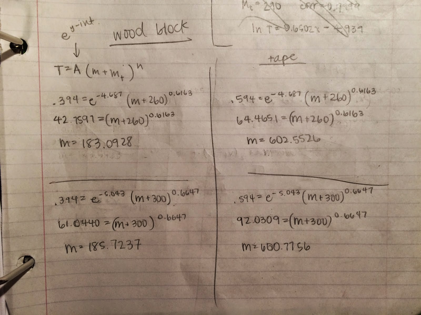
Figure 5: Calculations for unknown masses

Using the values derived from the steps above, we were able to calculate the masses of two objects by applying the mathematical model developed. The first object we used was an wooden block. By plugging in the values that we got of its period and the constants that we derived from before, we were able to find its mass to be 183.1 grams when considering M_tray to be 260 grams and 185.7 grams when M_tray was 300 grams. The next object that we tried to measure was a tape dispenser. We found its mass to be 602.6 grams when M_tray is set at 260 grams and 600.1 grams when M_tray is configured to be 300 grams. After we calculated the masses of the two objects theoretically, we used a scale to find the mass of the wooden block to be 180.2 and the mass of the tape dispenser to be 600.5 grams. Therefore, our mathematical model was relatively accurate.

CONCLUSION

From this experiment, we became familiar with the relationship between mass and period for an inertial balance. We learned that as the mass on an inertial balance increases, so does the time it takes for the inertial balance to complete two oscillations. In other words, when the mass becomes larger, the period does as well. We also learned that we can use this relationship to create a mathematical model that allows us to calculate unknown masses from their periods.

However, when we compared the theoretical and the measured values of these masses, we noticed that they were not a hundred percent accurate. This is to expected because we know that there are always number of factors that contribute to error in any given experiment. One of the possible factors that caused error in this particular experiment is that the added masses were not completely centered on the tray of the inertial balance. This could have altered the values that we got for the periods. Another source of error was that we did not pull back the same amount of distance before releasing the inertial balance during each trial. This also could have given us inaccurate period values.

Despite the number of reasons for error, we believe that the values were very accurate. This appears to be especially true when we consider all the limitations we had in this experiment. For example, we had no efficient way of keeping the masses steady when they were on the tray of the inertial balance except for by using tape. Therefore, we can conclude that this experiment was a relatively successful one.